Interferometry

Interferometer response function

Non-tracking interferometer

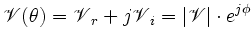
Figure 2.1: General geometry of a single baseline interferometer.

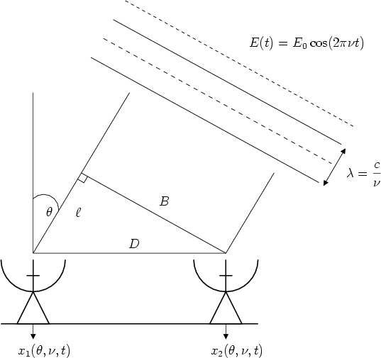A radio interferometer is a set of two or more antennas collectively used to measure the interference pattern produced by the angular brightness distribution of a very distant source at a given frequency. The vector connecting any pair of anntenas is called a baseline; its length defines the angular separation between regions of constructive and destructive interference and consequently, the resolution of the instrument. 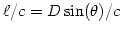The geometry of a single baseline interferometer is depicted in Figure 2.1. Two identical antennas are separated by a distance $D$. 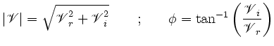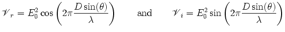An incident monochromatic plane wavefront $E(t)$, radiated by a distant point source located at an angle $\theta$ with respect to the normal of the baseline, will arrive at the leftmost antenna with a time delay of $\ell/c=D\sin(\theta)/c$, or equivalently, with a phase difference of $2\pi\ell/\lambda$. Let $x_1(t)$ and $x_2(t)$ be the electric signals induced at the output of each antenna. If the signals are combined according to the scheme described on Figure 2.2, then the normalized system output is given by:

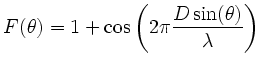$$F(\theta)=1+\cos\left(2\pi\frac{D\sin(\theta)}{\lambda}\right)$$ (2.1)

This expression is known as the Total power interferometer response function. Figure 2.3 presents a record of the transit of two "radio stars" obtained using this principle [Ryle et al., 1950]. Note that the interferometer used for this observations is a non-tracking interferometer which means that the antennas are not steered towards the source but instead they remain at a fixed position.

Figure 2.2: Left: Total power interferometer. Right: Top: Response function (equation 2.1) using a value of $D/\lambda =8$. Bottom: The same as before but considering the directivity $G(\theta )$ of the antennas assumed to be circular apertures with $R/\lambda \sim 1.2$. Compare with the observations of real point sources shown in figure 2.3

Figure 2.3: Record obtained using an east west total power interferometer. The sources are Cygnus A (16:20) and Cassiopeia A (19:30). (Taken form Ryle et al. [1950]). Compare with the total power interferometer response shown in figure 2.2.

Tracking interferometer

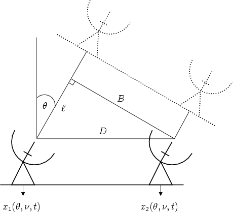
A more complex configuration known as multiplying interferometer is shown in figure 2.4. We see three major differences when compared with the previous one. First, an instrumental delay of $\tau_{g}=\ell/c$ has been included to compensate the geometrical delay, in other words, the phase center has been displaced to the direction $\theta$. Second, the antennas have been steered to the same direction. The interplay between delay and steering produces an "equivalent" interferometer whith a baseline of length $B=D\sin(\theta)$ as shown in figure 2.5. Finally, both signals have been split in two branches to form the in-phase and quadrature products. Both outputs are then combined in a single expression using complex notation:

$$\hbox{$\mathscr{V}$}(\theta)=\hbox{$\mathscr{V}$}_r+j\hbox{$\mathscr{V}$}_i=\vert\hbox{$\mathscr{V}$}\vert\cdot e^{j\phi}$$ (2.2)

where

$$\vert\hbox{$\mathscr{V}$}\vert=\sqrt{\hbox{$\mathscr{V}$}_r^2+\hb... ...phi=\tan^{-1}\left(\frac{\hbox{$\mathscr{V}$}_i}{\hbox{$\mathscr{V}$}_r}\right)$$

with

$$\hbox{$\mathscr{V}$}_r=E_0^2\cos\left(2\pi\frac{D\sin(\theta)}{\l... ... \hbox{$\mathscr{V}$}_i=E_0^2\sin\left(2\pi\frac{D\sin(\theta)}{\lambda}\right)$$

Figure 2.4: Multiplying interferometer.

Figure 2.5: General geometry of a single baseline tracking interferometer. The equivalent interferometer with an antenna separation of $B$ is shown in dotted lines (see the text for details).